The Birth of the BW Pathfinding Algorithm ( BWP )

The previous discussion

https://news.ycombinator.com/item?id=42608107

Ask HN: Have you ever seen a pathfinding algorithm of this type? | Hacker News

Hacker News

Explanation of the research process

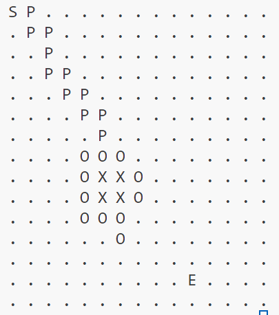
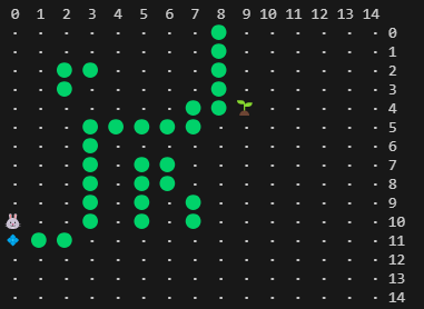
The basic approach is as follows:

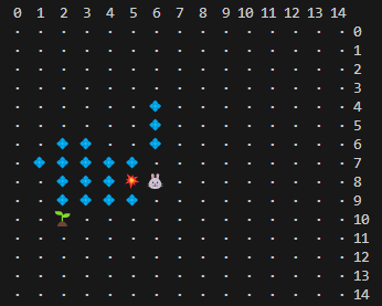
1. Determine the straight path from the starting point to the destination. (Utilizing Bresenham's Line Algorithm)
2. While calculating the path, if an obstacle is encountered, immediately stop and recognize the obstacle.
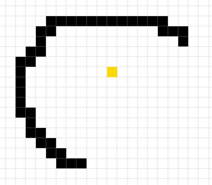
3. Retrieve the outline information of the obstacle.
4. Among the outline information, select the optimal point for bypassing the obstacle. (This part is the core)
5. Combine the starting point and the bypass point to create a kind of waypoint coordinate.
6. Subsequently, repeat the same process from the bypass point to the destination.
7. Ultimately, the path is constructed like this: (starting point, waypoint1, waypoint2, ..., waypointN, destination).

This is fundamentally the same concept as the ray concept used in 3D engines.
However, since I am working in a 2D context and diagonal movement is not allowed, I only made slight adjustments.

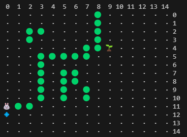
When obstacles were far away, it worked well according to the basic scenario.
However, when the obstacles were in close proximity, issues were identified.

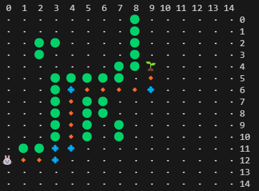
From here on, as the research is expected to be extensive, the debugging UX has been enhanced.

Therefore, in cases where obstacles are very close or the distance to the destination is short, I decided to apply different rules.
Since the computation load doesn't increase significantly and there aren't too many scenarios when the distance is short, we opted to try a somewhat brute-force approach.

In cases where either X or Y is a short distance, a brute-force yet simple approach was applied to evaluate the possible scenarios and find the path.

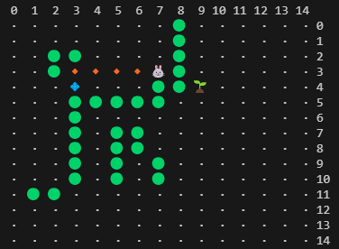
At this point, the rules were updated once again.
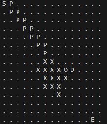
When encountering an obstacle, detecting the entire obstacle would be a waste of computation. Therefore, I wanted to switch to a method similar to how animals with vision behave, checking only the visible parts.

1. Detect a collision with an obstacle on the straight path connecting the starting point and the destination.
2. Decide which direction to explore along the obstacle's outline (for now, the side closer to the destination).
3. If the end of the visible outline is reached, search for an appropriate detour point around that outline.
4. Select a detour point where a straight-line movement from the starting point avoids the obstacle, preferably closer to the destination.
5. If the first detour point selection fails, I plan to search in the opposite direction along the outline where the obstacle was first encountered.

I applied the ideas developed so far and tested an algorithm that handles close-distance scenarios and selects detour points based on the line of sight.

After progressing to this point, I summarized the overall rules once again.

In general, for distances beyond a reasonable range, the following algorithm is applied:

• Calculate a straight path between the starting point and the destination using Bresenham's line algorithm.
• If an obstacle is encountered during the calculation, immediately stop the computation.
• Check the obstacles connected to the left and right of the detected obstacle based on its position.
• If the obstacles in a specific direction touch the map's boundary, exclude that direction.
• If both sides have open paths, calculate the positions of the obstacles visible at both ends in the field of view.
• Identify areas of available space near the ends and choose the corner with the largest available space as the next move target.
• If the available spaces are equal, choose the location closest to the starting point as the next move target.
• In certain cases, the path may get stuck at a sharp edge of an obstacle. In this situation, select the location near the obstacle where both the starting point and destination are close as the next move target.

If there are no obstacles from the beginning, the algorithm only needs to fire a single ray using Bresenham's line algorithm, ensuring the fastest performance. As the distance increases, the algorithm exhibits significantly higher performance compared to other algorithms (which, theoretically, is quite natural). By repeating the above process, the algorithm gradually finds its way to the destination.

For distances within a 10 x 10 range, a more simplified algorithm is applied:

• This algorithm accounts for cases where the path is in close contact with various obstacles in a narrow area.
• Starting from a distance of N, the algorithm decreases the distance by -1 while applying a simple method to navigate around obstacles.

In this case, the algorithm is simpler but may sometimes perform slower than A*.

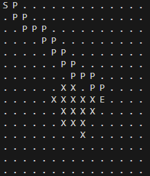
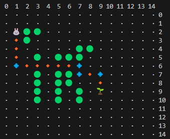
Now, I conducted tests to see if it could navigate much more challenging paths effectively.

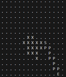
When obstacles are adjacent, detour points are selected too densely along the obstacle.

From this point on, a rule was applied to exclude dead-end paths, functioning somewhat like intuition. Additionally, it detects when obstacles continue in the same direction, enabling it to find the opposite detour point more quickly.

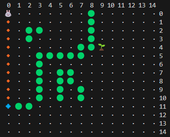
To be honest, this step feels more like a lucky break.
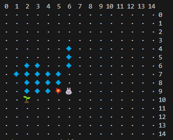
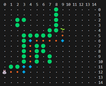
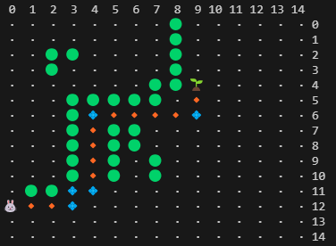
If it worked exactly as I implemented, it should have detected the obstacle extending downward, moved to (2,10), and then selected (0,10). But for some reason, it directly detected (0,10). While it works well as is and I’m leaving it that way, any developer would understand how terrifying it is to be in a "Why is this working?" situation.

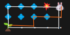
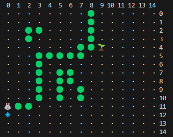
Finally, I compared the performance with the A* algorithm for long distances.
Keeping the starting point (7,3) and obstacle information unchanged, I only modified the destination to (100,100) and then checked the performance.
This means that once the visible obstacles above are cleared, the path to (100,100) is completely open.

This is something that anyone familiar with the principles of the A* algorithm could easily anticipate. And the method I am implementing only requires waypoints, so there is no need to calculate all the coordinate values as in A*. This also significantly contributes to performance improvement. The method I envisioned allows direct movement from (0,12) to (100,100). On the server, this computation is performed just once using Bresenham's Line Algorithm and then terminates. In Breathing World, this data is utilized to create visual effects on the client side. In Breathing World, the field of view can significantly exceed 1024, making the performance difference in this aspect immense.

Caught up in the joy of implementation, I hurriedly documented the process to the best of my memory.
There may be some missing details.
However, the code I wrote is publicly available, so feel free to take a look and share any feedback you may have!

The source code being maintained is here.
https://github.com/Farer/bw_path_finding

GitHub - Farer/bw_path_finding

Contribute to Farer/bw_path_finding development by creating an account on GitHub.

GitHubFarer

Development review

Now, I’d like to share some additional stories related to this research.

At first, I also used existing algorithms, most notably the A* algorithm. However, I eventually experienced situations where it didn’t deliver the performance I needed across a broader range of scenarios. This naturally led me to explore methods that could perform better. The idea actually started forming around January 9, 2024, approximately a year ago. Back then, my thoughts centered around the following:

https://qiao.github.io/PathFinding.js/visual/
https://movingai.com/GPPC/detail.html
https://www.movingai.com/benchmarks/grids.html
http://grastien.net/ban/articles/hg-icaps14.pdf
https://timmastny.com/blog/a-star-tricks-for-videogame-path-finding/

• Issue
  The shortest distance to the destination is a straight line drawn from the start to the endpoint. If this route is unobstructed, it’s the easiest and fastest way. However, the most significant issue arises when obstacles block this straight-line path.
  When there are obstacles, detours are necessary. From a human perspective, our “vision” allows us to detect distant obstacles and set an appropriate path accordingly. A* works differently, which creates the problem.
• Intuition
  One thing that sets humans apart from algorithms is what we often call "intuition." While existing methods couldn’t replicate this, AI, since the emergence of AlphaGo, seems to have started emulating what was previously thought to be a uniquely human trait.
  I believe that applying "intuition," which humans uniquely use for pathfinding, could make pathfinding significantly more efficient.
• Implementation (WIP)
  It might be worth leveraging the rays used in various game engines:

1. Compute the shortest path connecting the starting point and the destination.
2. Follow this path until you hit the first obstructed coordinate.
3. Identify the outline of the obstacle at that coordinate.

Back then, these were just ideas I had jotted down. Fundamentally, I wanted to implement pathfinding in a way that mimics how humans or animals navigate. That said, when I started developing Breathing World (BW), I naturally opted to use the A* algorithm, which I fine-tuned slightly into a Weighted A* algorithm for better performance.

A Bit About Breathing World

Currently, BW operates on ultra-low-power mini PCs powered by Intel’s N100 CPUs. 8 GB RAM and 256 GB SSD. This is to minimize fixed costs. Even though there are many affordable cloud services, operating the service from home with N100 mini PCs is still cheaper.
At present, the service runs on a total of 8 mini PCs, all physically located in South Korea.

Ultimately, I aim for a Global One Server architecture. How will I address service delivery to distant regions? For now, I’ve set up the service to target the Asia-Pacific region as a test.
To explain briefly, for regions far from South Korea, I operate relay and outpost servers. Relay servers run from my home, while outpost servers use the cheapest instances on Vultr’s cloud service—a $5/month plan. Those familiar with it would know this is one of the most affordable options available. Additionally, I’ve integrated bunny.net for static files like images.

I’ll cover BW’s server architecture in more detail in a separate post later.

Low Power, Human-Like Pathfinding

Given the constraints of using ultra-low-power CPUs for BW, I wanted to implement a method of pathfinding that’s lightweight and mimics how humans or animals find paths. Recently, I added wolves and expanded their vision, which led to performance issues—so I’ve been eager to try out this idea. Despite wrestling with various AI solutions and studying existing algorithms, I couldn’t find a satisfactory resolution.

After posting on Hacker News for input, I discovered several additional algorithms:

• Visibility Graph
• Incremental Search and Heuristics (ICAPS)
• Bug Algorithm

These algorithms implement pathfinding differently than A*. Though I couldn’t fully grasp every detail due to my limited technical knowledge, discussing them with AIs helped me understand their core concepts. Among them, the Bug algorithm fascinated me the most—it seemed quite similar to my approach.

I also learned that my method, in essence, aligns with modern research in robotics, where efficiency on low-spec hardware is especially critical.

I came across this recent study:
Finding Many Paths to a Moving Target

Insights and Reflections

One realization during this process is that many games implement pathfinding using the A* algorithm. If developers don’t optimize performance, they likely resort to higher hardware specs instead of exploring alternatives. This may explain why there hasn’t been much pressure to develop new methods.

After reviewing various algorithms, I observed their respective pros and cons. For example, performance may degrade with many obstacles or over long distances. Considering these factors, I concluded that using different methods for different scenarios might be the best solution.

Another key takeaway is that it’s unnecessary to find the entire path to the destination all at once. Finding a perfect path in one attempt requires preprocessing or high-performance hardware. For scenarios involving obstacles, you could simply identify a detour point, move there, and then calculate a new path to the destination.

Final Approach

I decided to divide cases into two categories:

1. When the range between the start and destination is within 10 x 10.
2. When the range exceeds this or involves very long distances.

Based on my performance measurements:

• For case 1, A* works well. Its efficiency is hard to surpass within a narrow range. However, my method has the advantage of being more intuitive—especially for those who dislike or struggle with mathematical reasoning, as A* can be difficult to grasp.
• For case 2, my method performs well because it models pathfinding akin to how humans or animals with vision navigate—intuitive and effective.

Closing remarks

I am not a super developer.
I am simply studying the parts necessary for the goals of the project I am working on.
Along the way, I achieved a small result, and I wanted to share it.
I also want to verify whether this is truly an achievement.
If there is anything I missed or did wrong, I would appreciate your feedback so I can make further improvements.
Thank you for taking the time to read this long post.

At that moment, I thought this was the end. 😅

Unfinished research ( 2025.1.31 )

I recently discovered that I had not applied a part of the A* algorithm implemented in .NET that could improve its performance.
In the A* source code, I had applied a SortedSet to the openSet section.
If this is replaced with a PriorityQueue, the performance will be significantly improved. So, I decided to apply this change and proceed with the tests again.
From this point onward, it would be better to focus on sharing performance results without including the map graphics for convenience. To ensure a more accurate comparison, I excluded the time taken to print logs in both cases.
I measured only the time purely spent on finding the path.
I also plan to expand the tests to cover longer distances and share those results.
You can focus on the time it took for the results.

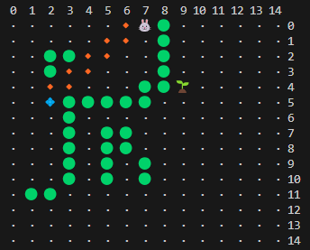
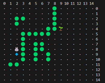
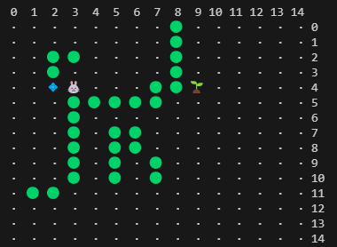
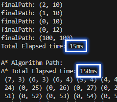
Start: (7, 3) -> Goal: (9, 4)
BW Total Elapsed time: 15ms
pathCase: reachableAlongOneDirection
finalPath: (7, 3)
finalPath: (3, 4)
finalPath: (2, 4)
finalPath: (0, 10)
finalPath: (0, 11)
finalPath: (0, 12)
finalPath: (3, 12)
finalPath: (3, 11)
finalPath: (4, 11)
finalPath: (4, 6)
finalPath: (9, 6)
finalPath: (9, 4)
A* Total Elapsed time: 3ms

Especially in cases where the path starts adjacent to an obstacle, A* appears to perform much better.
However, as mentioned before, the time difference is only 12 ms.

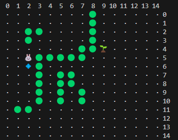
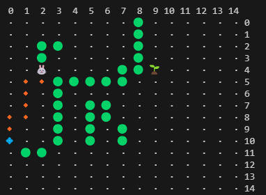
Start: (7, 3) -> Goal: (50, 50)
BW Total Elapsed time: 13ms
pathCase: reachableDirectly
finalPath: (7, 3)
finalPath: (3, 4)
finalPath: (2, 4)
finalPath: (2, 6)
finalPath: (2, 10)
finalPath: (1, 10)
finalPath: (0, 10)
finalPath: (0, 12)
finalPath: (50, 50)
A* Total Elapsed time: 5ms

However, there is an important point. The execution time of the algorithm I developed has decreased! And the rate of increase in the execution time of the A* algorithm has started to grow.
Of course, since the time differences are so small, there can be variations of about 0 to 2 ms each time the algorithm is run.

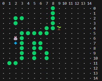
Start: (7, 3) -> Goal: (100, 100)
BW Total Elapsed time: 14ms
pathCase: reachableDirectly
finalPath: (7, 3)
finalPath: (3, 4)
finalPath: (2, 4)
finalPath: (2, 6)
finalPath: (2, 10)
finalPath: (1, 10)
finalPath: (0, 10)
finalPath: (0, 12)
finalPath: (100, 100)
A* Total Elapsed time: 6ms

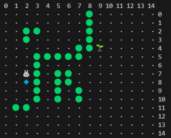
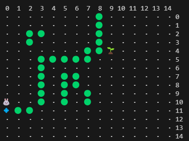
Start: (7, 3) -> Goal: (150, 150)
BW Total Elapsed time: 12ms
pathCase: reachableDirectly
finalPath: (7, 3)
finalPath: (3, 4)
finalPath: (2, 4)
finalPath: (2, 6)
finalPath: (2, 10)
finalPath: (1, 10)
finalPath: (0, 10)
finalPath: (0, 12)
finalPath: (150, 150)
A* Total Elapsed time: 10ms

The BW algorithm’s execution time decreased, while the A* algorithm’s execution time increased quite significantly.

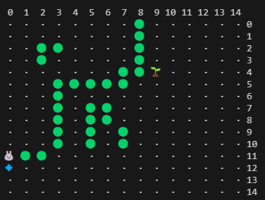
Start: (7, 3) -> Goal: (200, 200)
BW Total Elapsed time: 13ms
pathCase: reachableDirectly
finalPath: (7, 3)
finalPath: (3, 4)
finalPath: (2, 4)
finalPath: (2, 6)
finalPath: (2, 10)
finalPath: (1, 10)
finalPath: (0, 10)
finalPath: (0, 12)
finalPath: (200, 200)
A* Total Elapsed time: 18ms

Aside from being surrounded by obstacles near the starting point, it's just a wide-open path. However, as mentioned repeatedly, this is because the Bresenham's line algorithm allows for movement in a straight line all at once. It’s based on a very simple principle.
Now, let's take a look at the results for even longer distances.

Start: (7, 3) -> Goal: (250, 250)
BW Total Elapsed time: 13ms
pathCase: reachableDirectly
finalPath: (7, 3)
finalPath: (3, 4)
finalPath: (2, 4)
finalPath: (2, 6)
finalPath: (2, 10)
finalPath: (1, 10)
finalPath: (0, 10)
finalPath: (0, 12)
finalPath: (250, 250)
A* Total Elapsed time: 37ms

Start: (7, 3) -> Goal: (300, 300)
BW Total Elapsed time: 12ms
pathCase: reachableDirectly
finalPath: (7, 3)
finalPath: (3, 4)
finalPath: (2, 4)
finalPath: (2, 6)
finalPath: (2, 10)
finalPath: (1, 10)
finalPath: (0, 10)
finalPath: (0, 12)
finalPath: (300, 300)
A* Total Elapsed time: 48ms

When finding a path on an open road, you can see that BWP maintains consistent performance as the distance increases. On the other hand, A*'s performance gradually decreases.
This shows that when trying to expand the wolf’s field of view and move over longer distances, the performance drops significantly.

Advanced Testing

From this point onward, we will conduct tests for cases where each destination is surrounded by obstacles.
For this test, I created a 301 x 301 image file using Paint.Net.

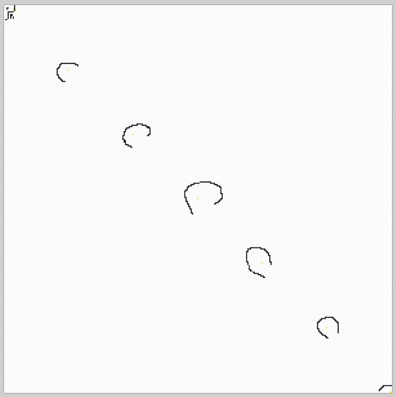
If BWP performs better than A* in this scenario as well, it truly means I have achieved my intended goal.

Start: (7, 3) -> Goal: (50, 50)
BW Total Elapsed time: 14ms
pathCase: reachableAlongOneDirection
finalPath: (7, 3)
finalPath: (3, 4)
finalPath: (2, 4)
finalPath: (2, 6)
finalPath: (2, 10)
finalPath: (1, 10)
finalPath: (0, 10)
finalPath: (0, 12)
finalPath: (40, 50)
finalPath: (40, 49)
finalPath: (40, 48)
finalPath: (41, 47)
finalPath: (42, 46)
finalPath: (42, 45)
finalPath: (43, 44)
finalPath: (55, 44)
finalPath: (58, 45)
finalPath: (58, 50)
finalPath: (50, 50)
A* Total Elapsed time: 7ms

Start: (7, 3) -> Goal: (100, 100)
BW Total Elapsed time: 16ms
pathCase: noPath
finalPath: (7, 3)
finalPath: (3, 4)
finalPath: (2, 4)
finalPath: (2, 6)
finalPath: (2, 10)
finalPath: (1, 10)
finalPath: (0, 10)
finalPath: (0, 12)
finalPath: (40, 50)
finalPath: (40, 49)
finalPath: (40, 48)
finalPath: (41, 47)
finalPath: (42, 46)
finalPath: (42, 45)
finalPath: (43, 44)
finalPath: (55, 44)
finalPath: (58, 45)
finalPath: (91, 102)
finalPath: (91, 101)
finalPath: (91, 100)
finalPath: (92, 99)
finalPath: (92, 97)
finalPath: (93, 96)
finalPath: (93, 95)
finalPath: (94, 94)
finalPath: (96, 93)
A* Total Elapsed time: 21ms

I was slightly thrown into a state of panic.
After spending so much time and effort, how could this situation arise!

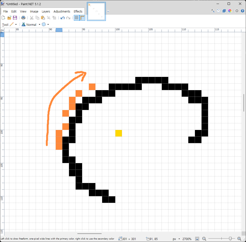
It is very good that the algorithm successfully identifies distant obstacles and selects appropriate detour points as intended.
However, it is clear that the logic for finding detour points after that is flawed.

When the destination is at 50,50, it did succeed in reaching the destination, but I also noticed that the path similarly backtracked after encountering an obstacle.

Once again, I fell into deep anguish.

Algorithm Improvement ( 2025.2.3 )

After selecting the first detour point for a distant obstacle, I modified the algorithm so that when choosing the next detour point, it takes into account the relative position from the previous point to ensure it doesn't backtrack against the intended direction of progress.

Final internal testing ( 2025.2.5 )

I would now like to share the results of testing conducted on the actual LIVE server.
The server hardware specs are based on a Mini PC using the ultra-low-power Intel N100 CPU.
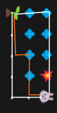
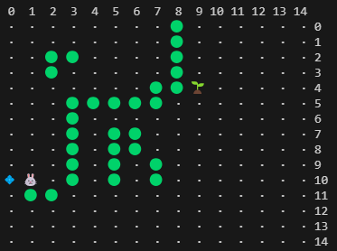
Since the BWP path is short, the entire path is being displayed together.
This is the final internal testing result.

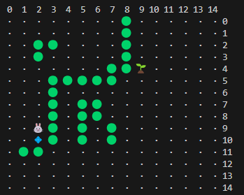
BW Path
(7, 3)
(2, 5)
(0, 10)
(0, 11)
(0, 12)
(3, 12)
(3, 11)
(4, 11)
(4, 6)
(9, 6)
(9, 4)

Start: (7, 3) -> Goal: (9, 4)

BW Path Count: 11
BW Total Elapsed time: 31ms

A* Path Count: 34
A* Total Elapsed time: 7ms

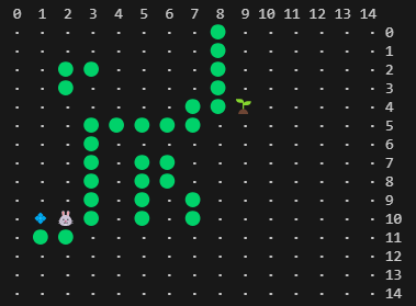
BW Path
(7, 3)
(2, 5)
(0, 10)
(0, 11)
(0, 12)
(56, 44)
(58, 45)
(58, 50)
(50, 50)

Start: (7, 3) -> Goal: (50, 50)

BW Path Count: 9
BW Total Elapsed time: 31ms

A* Path Count: 121
A* Total Elapsed time: 14ms

BW Path
(7, 3)
(2, 5)
(0, 10)
(0, 11)
(0, 12)
(56, 44)
(111, 92)
(113, 93)
(114, 94)
(113, 94)
(114, 95)
(114, 96)
(114, 101)
(113, 102)
(100, 100)

Start: (7, 3) -> Goal: (100, 100)

BW Path Count: 15
BW Total Elapsed time: 32ms

A* Path Count: 227
A* Total Elapsed time: 43ms

BW Path
(7, 3)
(2, 5)
(0, 10)
(0, 11)
(0, 12)
(56, 44)
(113, 93)
(160, 136)
(164, 138)
(166, 139)
(168, 140)
(169, 141)
(170, 145)
(170, 146)
(170, 147)
(170, 151)
(169, 152)
(168, 153)
(167, 154)
(165, 155)
(150, 150)

Start: (7, 3) -> Goal: (150, 150)

BW Path Count: 21
BW Total Elapsed time: 34ms

A* Path Count: 331
A* Total Elapsed time: 87ms

BW Path
(7, 3)
(2, 5)
(0, 10)
(0, 11)
(0, 12)
(56, 44)
(113, 93)
(166, 138)
(168, 139)
(203, 188)
(205, 190)
(206, 191)
(207, 193)
(208, 198)
(208, 199)
(208, 200)
(208, 202)
(200, 200)

Start: (7, 3) -> Goal: (200, 200)

BW Path Count: 18
BW Total Elapsed time: 33ms

A* Path Count: 425
A* Total Elapsed time: 149ms

BW Path
(7, 3)
(2, 5)
(0, 10)
(0, 11)
(0, 12)
(56, 44)
(113, 93)
(168, 139)
(256, 241)
(258, 243)
(260, 245)
(260, 246)
(260, 247)
(260, 255)
(250, 250)

Start: (7, 3) -> Goal: (250, 250)

BW Path Count: 15
BW Total Elapsed time: 33ms

A* Path Count: 527
A* Total Elapsed time: 216ms

BW Path
(7, 3)
(2, 5)
(0, 10)
(0, 11)
(0, 12)
(56, 44)
(113, 93)
(168, 139)
(256, 241)
(295, 294)
(293, 295)
(292, 296)
(291, 297)
(290, 298)
(290, 300)
(300, 300)

Start: (7, 3) -> Goal: (300, 300)

BW Path Count: 16
BW Total Elapsed time: 34ms

A* Path Count: 605
A* Total Elapsed time: 60ms

BW Path
(7, 3)
(2, 5)
(0, 10)
(0, 11)
(0, 12)
(1920, 1080)

Start: (7, 3) -> Goal: (1920, 1080)

BW Path Count: 6
BW Total Elapsed time: 27ms

A* Path Count: 3005
A* Total Elapsed time: 632ms

Unverified Cases

• When there are extremely complex obstacles from the starting point to the destination
• Finding an exit in a complicated maze

Currently, BW doesn’t have such cases, so I haven't conducted tests for them yet.

In fact, for these scenarios, simply using A* would likely be the best approach (especially when the distance is short). I plan to modify BW later to use A* when dealing with short-distance pathfinding.

However, since BW only needs to extract waypoint-based coordinates, I will proceed with the current implementation for now.

Deploy to the LIVE server ( 2025.2.6 )

Finally, I decided to deploy it to the LIVE server.
The process of merging it with the existing source code wasn’t entirely smooth, but since I had structured the development systematically, I was able to complete the integration without major issues—something I felt quite proud of.

And then, the monitoring began.

[ Error ] FindExtremeAngleTargets - No leftmost or rightmost target found.
No leftmost or rightmost target found.
Origin: (9025, 11968)
Origin: (9071, 11865)
targets: System.Collections.Generic.List1[System.ValueTuple2[System.Int32,System.Int32]]
isReachable: True
angles: System.Collections.Generic.List1[System.ValueTuple2[System.Double,System.ValueTuple`2[System.Int32,System.Int32]]]

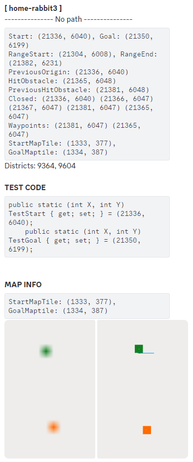
--------------- No path ---------------
Start: (25599, 12431), Goal: (25624, 12408)
RangeStart: (25576, 12376), RangeEnd: (25656, 12456)
StartMapTile: (1599, 776), GoalMaptile: (1601, 775)
HitObstacle: (25616, 12416)
PreviousHitObstacle: (25616, 12417)
Closed: (25608, 12424) (25599, 12431) Closed: System.Collections.Generic.HashSet1[System.ValueTuple2[System.Int32,System.Int32]]
PreviousOrigin: (25599, 12431)
Waypoints: (25608, 12424) (25599, 12431)

As expected, the worst-case scenario became a reality.
The war against bugs had officially begun.

If you look at the logs above, you’ll see that in BW, the coordinate system for animals covers an extremely vast range.
The coordinate range for plants is 1920 x 1080 = 2,073,600.
Animals, however, have a much finer resolution—each plant coordinate is further divided into 16 x 16 units.
This results in a total range of: 1920 x 16 x 1080 x 16 = 530,841,600.

The reason for this design choice was to achieve a more precise representation of animal positions. Naturally, this led to significantly large coordinate values.

And that’s what ultimately led me to research and develop the BWP algorithm.

At first, I focused on logging coordinate values, but I quickly hit the limits of debugging this way. So, I decided to develop a notification system specifically for debugging.
From this point on, most of the bugs I encounter will be LIVE server-specific—just something to keep in mind.

The debugging system development is complete. ( 2025.2.18 )

After weeks of battling bugs, I’ve finally completed the development of the debugging system.

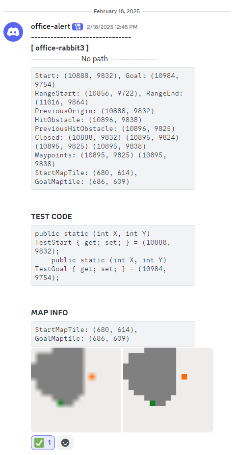
Even if the path is not found immediately, it’s not a huge issue. However, whenever the path cannot be found, a notification is always triggered.
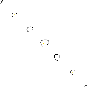
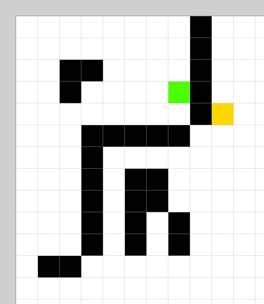
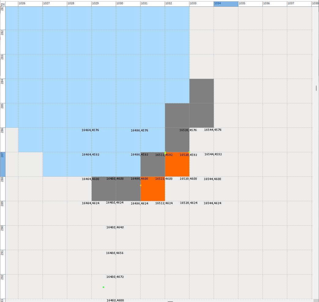
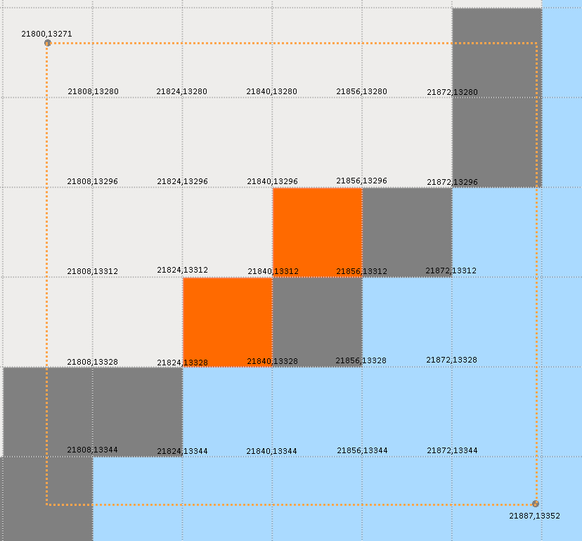
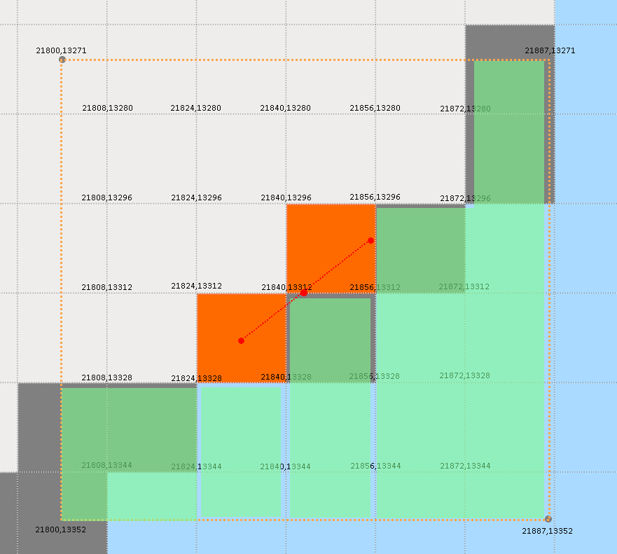
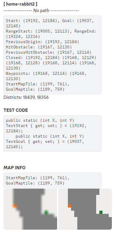
The system generates an image file with the coordinates at that moment, along with surrounding map and terrain information, and sends it along with the notification.

The TEST CODE section is prepared to be directly pasted into the code at https://github.com/Farer/bw_path_finding.

At first, I would transfer the code there, replicate the same situation, and proceed with debugging. Later on, I decided to just prepare the test code directly in the LIVE server code and continue debugging from there.

I'm getting close to the final completion. ( 2025.2.24 )

After countless rounds of debugging, now only the following error cases occur:

In such cases, increasing the search range might help find the path, but it would also result in significantly more computations, which doesn't align with the BWP concept. BWP is built on the premise that there may be situations where a path cannot be found. If it can’t be found the first time, the path can be searched again when the situation changes.

The key point is to minimize the computations when trying to find a path. Later on, in these cases, the system might move to a different location instead of staying at the current one, and upon re-evaluating the situation, it could find another weed. This could lead to the goal changing to a much faster reachable point.

It’s similar to how a person, after visually or intuitively assessing a path, would change their position if they couldn't find a solution, just to try a different approach.

In this case, it was found that a tree is blocking a large area near the starting point. However, this isn’t a major issue because, next time, the system will attempt to find a weed at a different location.

At this point, the starting point can be slightly adjusted, and the system can track weeds again based on the changed situation. This way, the pathfinding process remains flexible and adaptable to new conditions.

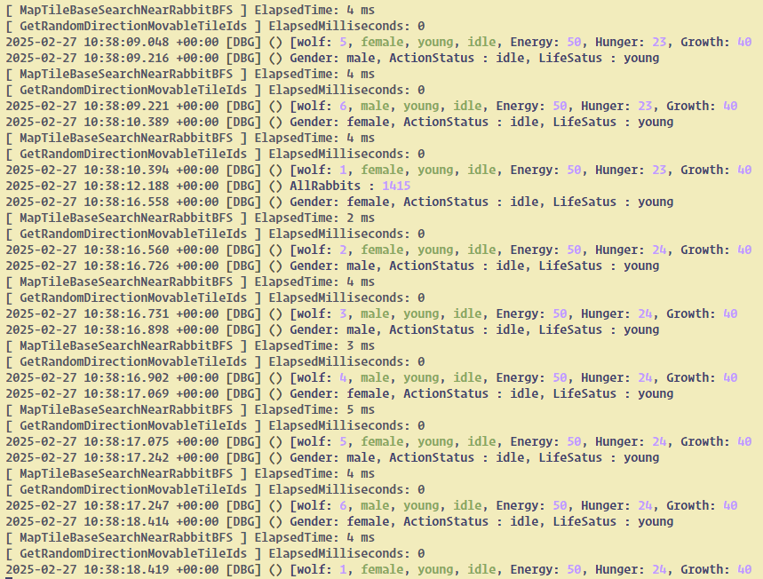
The return of the wolf! ( 2025.2.27 )

Finally, the problematic wolf has returned!

Originally, I expanded the wolf's vision and used A* for rabbit tracking and movement, but due to performance issues, I started this research.

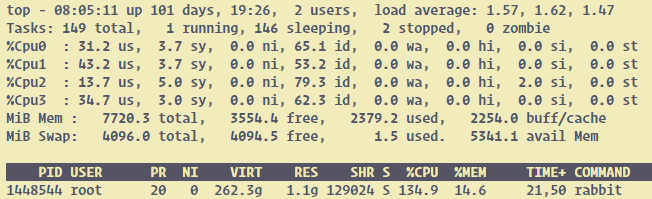
Here, I’d like to share the results of the performance monitoring from the current LIVE server.

Dashboard - Breathing World

Breathing World

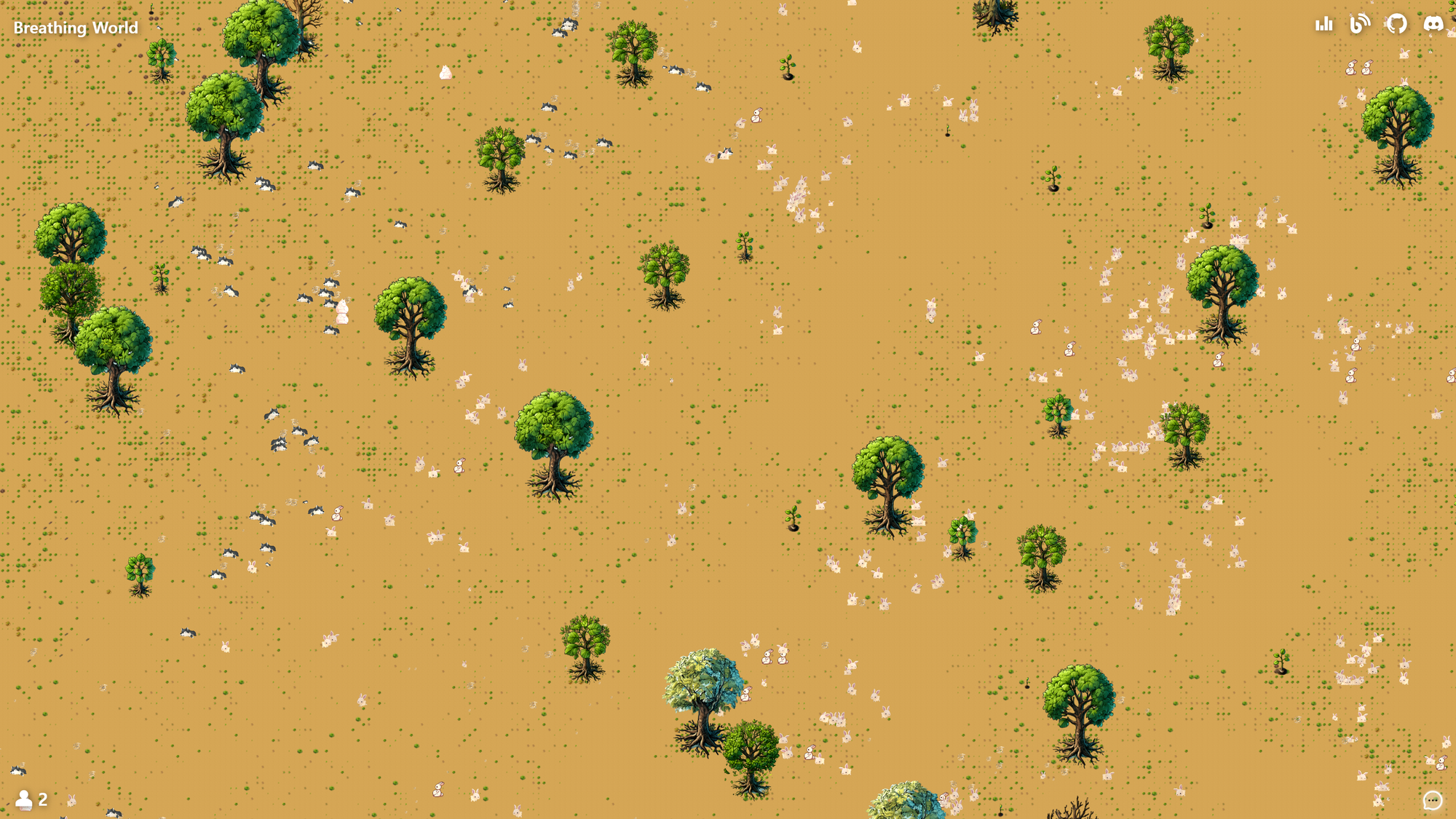
If you visit the page, you’ll be able to see a dashboard like the one below.

Currently, five servers are running smoothly: plants (weeds/trees), rabbit1, rabbit2, rabbit3, and wolf1. Each server automatically adjusts the number of entities based on the population. This reflects the core concept of the BW project—an ecosystem cycle.

There are three rabbit servers, and each server adjusts its maximum number of entities based on its performance. In other words, using a higher-spec server allows for processing a much larger number of entities. However, this directly impacts maintenance costs, so I’m currently trying to optimize performance on the Intel N100 CPU.

As I mentioned earlier, I’d like to dedicate a separate post to discuss the details of the BW server.

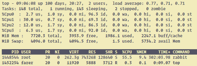
In the case of the rabbit server, even with over 1,000 rabbits, the server load has significantly decreased compared to before. Although I don’t have any old screenshots, previously, with around 1,000 rabbits, the load was about 2 to 3 times higher than it is now.

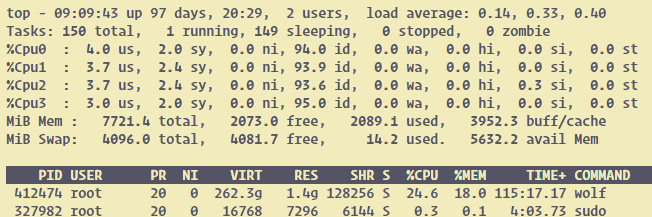
The wolf server is also running very stably now. Currently, there are only about 200 wolves, but in the past, even with this many, the rabbit and pathfinding calculations would spike, causing constant freezes. Given the current ecosystem dynamics, it’s unlikely for the wolf population to surge dramatically, so I plan to continue operating with a single server for now. Similar to the rabbit server, the wolf server is designed to be easily scalable, allowing additional servers to be added whenever needed.

The current version of the wolf is still in the draft phase, so its hunting skills are poor, and it doesn’t have a unique lifestyle yet. Now that the core technology is complete, I’ll soon be working on refining and enhancing the wolf’s lifestyle.
https://blog.breathingworld.com/concept-meeting-for-wolf-development-with-gpt/

This is truly the final word.

First of all, I’d like to sincerely thank anyone who has taken the time to read this long post with interest. Until now, I’ve only been reading articles in technical communities, but I wanted to muster up the courage to write something myself. While I may not be making a groundbreaking mark in the history of pathfinding algorithms, I’ve achieved considerable progress in my project, and I hope this could provide a new perspective on algorithms for those who are interested.

The BW project will continue, and I believe you’ll be able to check its progress at any time. After almost two years of contemplation and about three months of intense research, I feel a personal sense of pride in the results I’ve achieved.

If anyone continues to take interest in the BW project, my basic ambition is to continue showcasing the evolution of the ecosystem as it grows more sophisticated.

Additional Note

It truly seems like a great era for developers to collaborate with AI. I’d also like to express my gratitude to the many AIs that have been part of this research.

Real Last Performance Report